How HeatWise Works

HeatWise uses the Radiant Time Series (RTS) calculation procedure for calculating cooling loads. Below is a high-level overview of how the loads are actually calculated. For a detailed comparison between different cooling load calculation methods, see our blog post on HVAC load calculation method comparisons.

A Quick Comment on Heating Loads

Although energy used for heating is often more intensive and more important than cooling, the process of calculating heating loads is fairly simple, and will not vary much between software options.

Heat loads are calculated by looking at envelope conduction and infiltration for each exterior zone, and then adding in any ventilation load. For heating load calculations, it is assumed that there are no internal loads producing heat, and no thermal storage of the building to take away from instantaneous conduction.

Space Cooling Load Calculations

The first part of computing the total system cooling load is to build a matrix of sensible and latent results for each space, where each entry represents the cooling load for a particular hour and month for that space.

The contributors to the cooling load are first split into sensible and latent components, each of which is treated separately.

Sensible Cooling Loads

The sensible loads can be arranged into three categories:

1. Envelope conduction
2. Solar gains
3. Internals

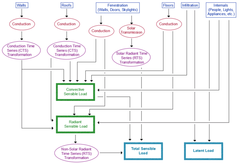
In addition to this breakdown, the envelope conduction and the internals are further split into convective and radiant (non-solar) portions. The image below shows the full breakdown and calculation procedure for each space at a particular month and hour:

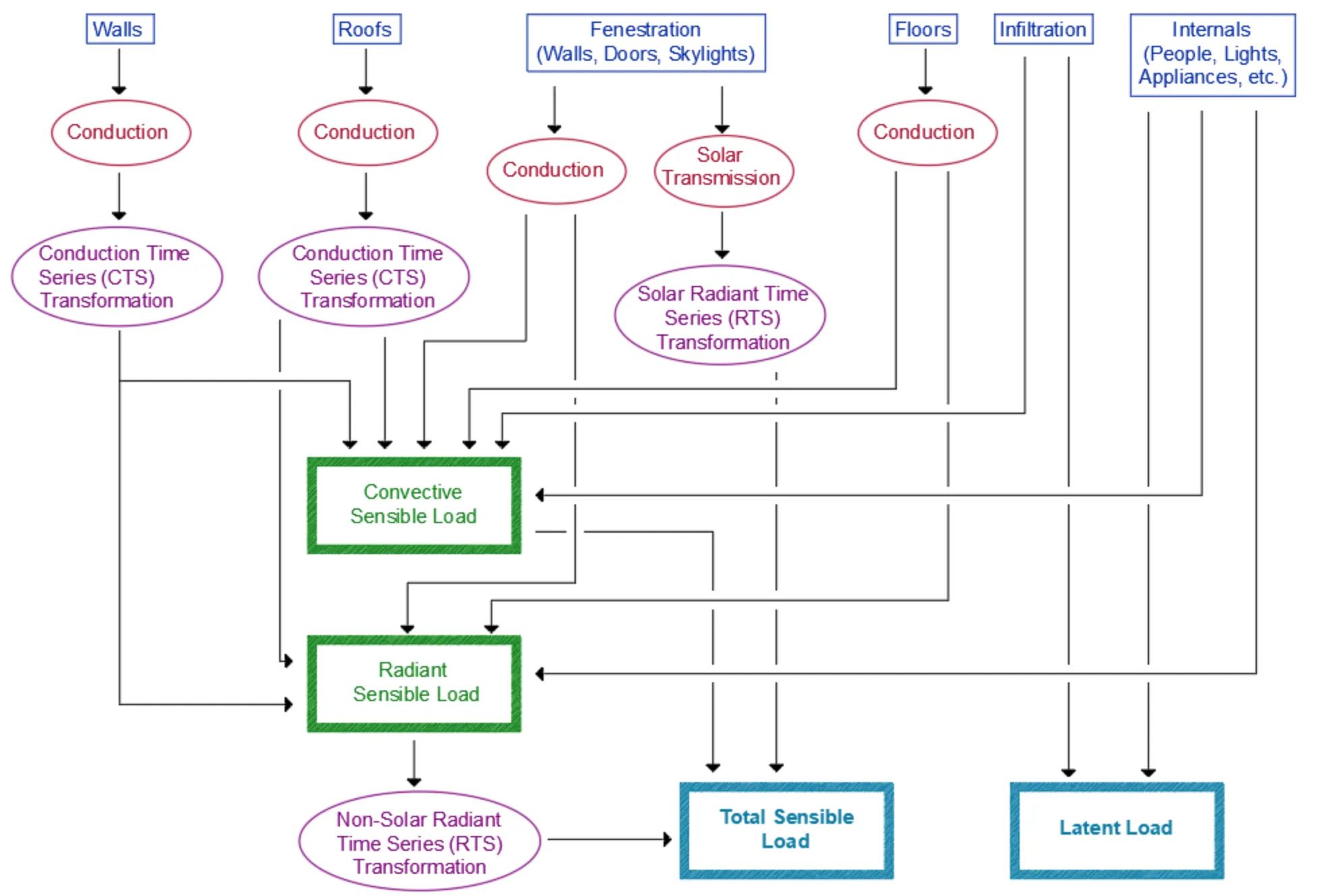The first item to note here is that both walls and roofs go through a Conduction Time Series (CTS) transformation. This is a linear transformation of a daily load profile on each wall and roof in the space. This transformation applies a time delay to the peak loads due to heat absorption and gradual release by the building materials. The nature of the time delay is dependent on the wall type and thermal mass. It should also be noted that some floor types do not contribute to the cooling load, and those that do contribute do not go through a CTS transformation.

The CTS time delay is not applied to fenestration products. Instead, fenestration is spilt into two kinds of cooling load: conduction and solar gains. Conduction will happen at any hour and is only a function of temperature difference across the glass, whereas solar gains are a function of solar angle, internal shading, external shading, and glass characteristics.

Internal loads from lights, people, appliances, etc. are dependent on the characteristics of each item and can be highly variable. HeatWise has built-in specifications for heat gain from many different types of internal loads for accurate heat gain calculations.

Infiltration will also contribute to the sensible cooling load, however it is 100% convective and is therefore directly combined with the other convective portions of heat gains.

Convective Versus Radiant Sensible Loads

The sensible cooling loads from walls and roofs (after CTS transformations), and from floors, fenestration and internals are then split into convective and radiant portions. The percentage of each element that is assigned as radiant versus convective is different for each cooling load component, and HeatWise uses the recommended values published in the ASHRAE Fundamentals Handbook.

The convective portion from each element is assumed to immediately enter the air and contribute to the instantaneous cooling load. The radiant portion is assumed to be absorbed by building materials and slowly released overtime, creating a time delay similar to the CTS time delay described above. However, this time delay is dependent on the amount of glass in the space, the weight of building construction and furniture, and whether the space has a carpet or hard floor. The radiant non-solar loads are put through a Radiant Time Series (RTS) linear transformation, which is the exact same as the CTS transformation but with different time delay characteristics. The RTS non-solar delay is applied to both internal and external zones, and is different for each space depending on the space characteristics.

The solar loads through the fenestration are then put through a solar RTS transformation, which is the same as the non-solar kind except with different numbers to reflect the different nature of the radiation.

Once the transformed radiant values are obtained, they can be added to the convective values (including infiltration) to obtain a total space sensible cooling load for each hour.

Latent Cooling Loads

Latent loads in a space can only come from internal elements and infiltration. Latent loads are entirely convective, so there is no time delay applied to them, making them straightforward to calculate.

Space Airflow Calculations

Space airflow is calculated based on the sensible load at any given time. In a CAV system, the peak cooling load is used to calculate the airflow for the space. In a VAV system, airflow will vary at all hours, however it must always be at or above its minimum. The minimum airflow is calculated by $V_{pz-min}=1.5 \times V_{oz}$, where $V_{oz}$ is the outdoor air required for that space, as calculated by part 6 of ASHRAE Standard 62.1. Airflow at any given time is then calculated by: $Q_{space}=\frac{q_{space}}{60\times0.24\times\rho_{air}\times(T_i-T_s)}$

Where $Q_{space}$ is the airflow to the space, $q_{space}$ is the cooling load of the space at the hour being calculated, $\rho_{air}$ is the density of the air, $T_i$ is the internal zone temperature and $T_{s}$ is the supply air temperature.

In situations of a CAV system where the heating airflow (calculated in a similar way) is higher, then that airflow is used for the zone instead of the cooling airflow when analysing the system as a whole.

Coil Load Calculations

Once the airflow for each zone is known, the total system airflow can be calculated by taking the sum of all zones. The coil sensible and latent loads can then be calculated using the equations below: $q_{sens}=Q_{total}(60\times0.24\times\rho_{air})\times(T_m-T_s)$

$q_{lat}=Q_{total}(60\times\rho_{air})\times(W_m-W_s)\times(1061+0.444T_{avg})$

Where $T_m$ is the mixed air (ventilation + return air) temperature, $W_m$ is the mixed air humidity ratio [lb_water/lb_{dry air}], $W_s$ is the supply air humidity ratio, and $T_{avg}$ is the average temperature in the cooling process (average of $T_m$ and $T_s$).

The values of $T_m$ and $W_m$ come from the psychrometric state of return air mixed with the ventilation air, which is dependent on whether or not an ERV and/or an economizer is used. The image below shows a diagram of how the coil load calculations work, once the space load calculations have been completed.

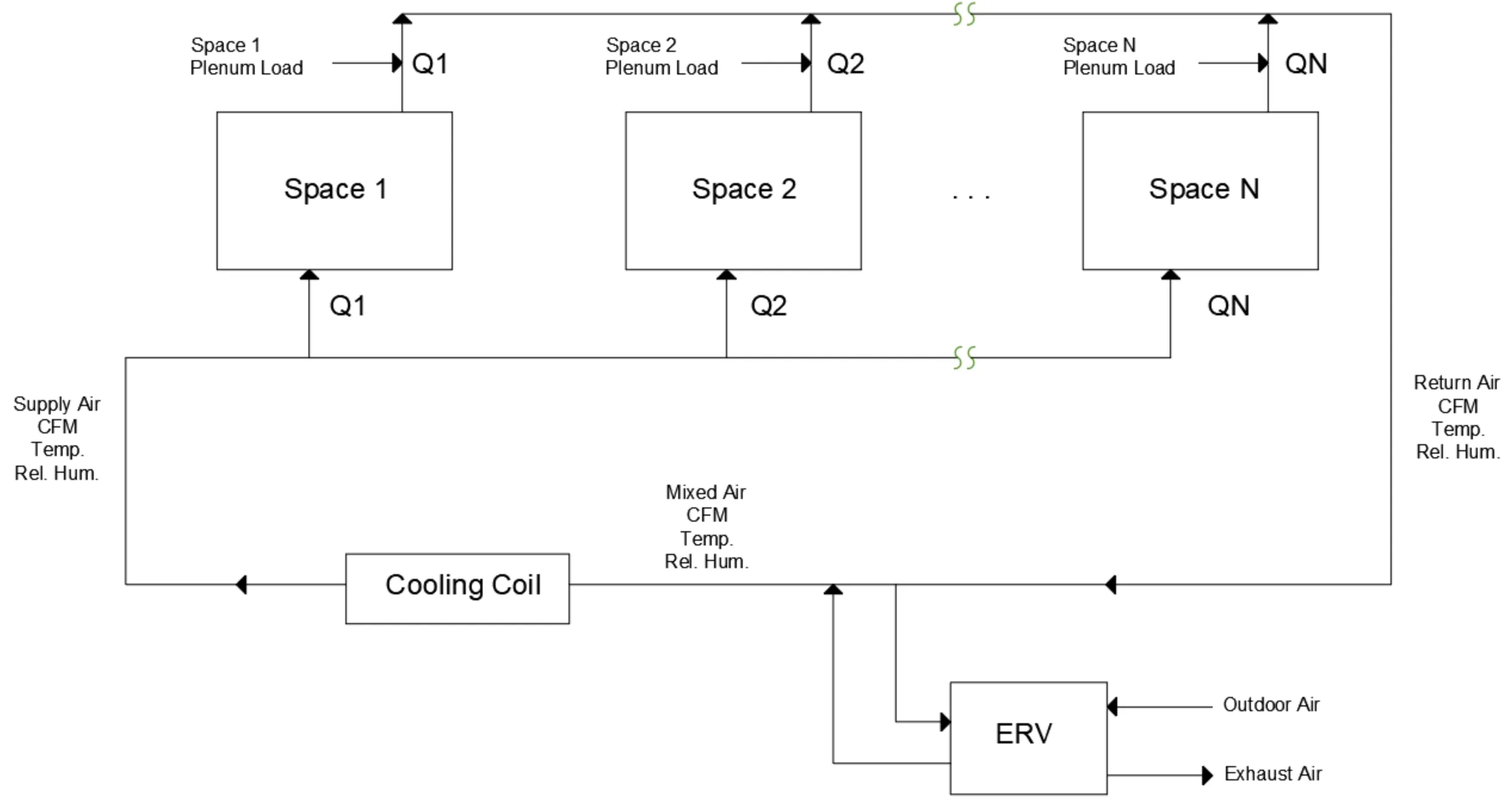In the above diagram it shows that the airflow going into a space is equal to the airflow coming out. Return air will be at the state of the space (temperature and humidity), except with the possible additional plenum loads. For more information on how the plenum load for each space is calculated and how it can affect the return air temperature, see our blog post on Plenum Load Impacts.

Conclusion

There are additional complexities in the calculation of space and system loads, but the descriptions above give an overview of the general process. The process starts with space load calculations, which include the CTS and RTS transformations. Those space loads determine airflow and ventilation requirements for each space and the system as a whole. Then the total airflow is simulated going across the cooling coil with a return temperature and humidity that is dependent on the system setup (heat recovery, economizer, etc.).

To see how HeatWise compares to other software, see our blog post comparing different options for HVAC software.