Radiant Time Series (RTS), Cooling Load Temperature Difference (CLTD), and Heat Balance are different methods of obtaining the same goal: calculating the total cooling load in a space. As research has improved over the years, and as computers have become more powerful and accessible, methods of performing cooling load calculations have evolved. For many decades, ASHRAE’s Fundamentals Handbook, which is published every four years, would give a detailed description of how to perform cooling load calculations based on current knowledge and capabilities in the field of HVAC. However, in the 1997 edition of the Fundamentals Handbook, ASHRAE included a new calculation method: Radiant Time Series.
Through many iterations of the Fundamentals Handbook, ASHRAE has given their detailed process for performing load calculations, whether CLTD or RTS, in addition to a full breakdown of the Heat Balance method (HB). The HB method is the most mathematically sound and complete method for performing load calculations - it is a full description of all thermal energy transfer into and out of each surface of a space. However, it is also the most computationally intensive by a significant margin.
Cooling load calculations are given greater weight than heating load calculations within HVAC design for two primary reasons: Cooling load calculations are far more complicated. Accuracy is more important in cooling load calculations.
Oversizing heating equipment usually has a very small impact on project capital costs, and almost no impact on operating costs. The reason oversizing heating equipment does not impact operational costs is because heating is achieved in two primary ways: Electric resistance heat Carbon-based fuel
With both of these methods the impact of oversized equipment just means that more heat will be added to the space when the equipment is on, but the amount of heat output versus input will have little to no change. The net result will likely be additional cycling of the heating elements, which is usually not a big deal, and will have little impact on efficiency (as long as it’s not to an extreme degree).
Oversizing your cooling equipment means it will operate below its peak performance even at peak times, and therefore it will operate far below its peak performance during off-peak times. This is because of the complexity of using a refrigeration cycle to move thermal energy compared to simple electric resistance or the burning of fuel. When cooling equipment is operating at a sub-optimal point on its efficiency curve, the net cooling effect versus net energy input will decrease, causing higher electricity costs compared to the net benefit. With all of the complicated variables involved in calculating cooling loads, the risk of oversizing equipment becomes significantly larger, and the magnitude of the oversizing will increase as well.
In its purest form, the HB method considers every surface in a room, including surfaces of people, equipment, and furniture. It considers the radiant heat exchange between all surfaces with each other, as well as between all surfaces and the room air.
For the building envelope, the HB method calculates the heat flux on the exterior and interior surfaces of all walls, roofs, windows, etc., as well as the heat being absorbed or released by these building features. It also considers heat being absorbed and released over time of the furniture and building materials in a room. By doing this, it accounts for the total flow of all energy in a room over time. The only thing not typically modelled is the air in the room, which is usually assumed to be well-mixed and slow-moving. To fully model the room air, computational fluid dynamics (CFD) would need to be used in addition to the load calculations, adding additional computational resources required to perform the full simulation.
This method typically uses a 12-month, 24-hour daily simulation to gain accurate results on the timing of concurrent loads and the process of heat absorption and release by the building. Taking all of these variables into account makes the HB method extremely complicated, and where spaces are large with many internal loads, it becomes very time consuming and expensive.
Figure 1 below is a schematic of the calculation methodology for the HB method. Although this does not look overly complicated, take note of the words “DUPLICATE FOR EACH SURFACE” in the bottom right corner of the grey rectangle. This means that the calculations contained in the grey rectangle must be performed for all surfaces enclosing the space (ceiling, walls, floors, windows, etc.), and the radiative interactions of every surface with every internal source must be calculated.
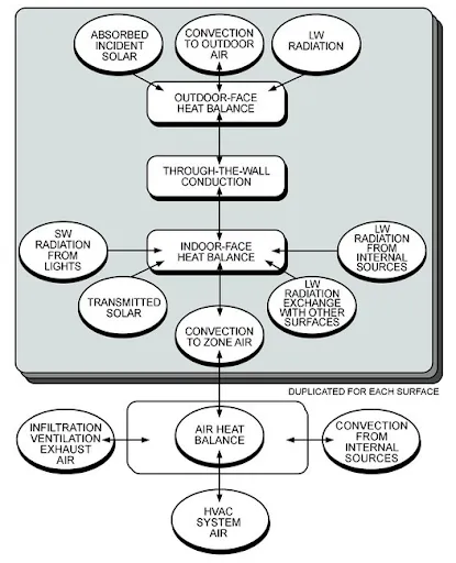 Figure 1: Heat Balance Schematic [1]
The CLTD method is highly simplified and outdated. It is simple enough that it can be modelled by most engineers by using a spreadsheet. This makes it useful for small, single-space buildings where the user wants full control of the calculations and variables. However, with increasing size and complexity of the building and systems, the CLTD method tends to overestimate loads, and its capability for refining results with increased knowledge of the building is limited.
Each item in the space that contributes to the cooling load, such as walls, people, etc., is assigned a CLTD value, which comes from tables published by various researchers and is presented by ASHRAE in the older handbooks. These values will vary depending on factors like wall exposure direction, activity level of the occupants, etc., however it does not go through a full year simulation in the same way that the HB and RTS methods do.
The CLTD method was a useful tool for a long time. However, with modern computers and commercial HVAC software, it has become outdated. The one advantage of the CLTD method is that it is “static”, meaning you do not necessarily need your computer to run through hundreds or thousands of iterations to obtain your loads.
The RTS method is a good stepping stone between CLTD and HB calculation methods. The RTS method takes advantage of hourly load profiles of outside temperature, solar radiation, appliance use, occupancy, and more, similar to the HB method. Where the HB method considers the interactions between all surfaces in the space, the RTS method simply applies a time delay for each load based on statistical data from research projects. This is done in three parts:
CTS time delay is applied to the walls and roofs. It makes estimates based on the type of building construction and the wall or roof mass. RTS non-solar time delay applies only to the radiant portion of non-solar sensible loads. All loads from the building envelope and from internal sources can be split into convective and radiative portions; the convective portion is immediately added to the room cooling load, whereas the radiative portion is first transformed under the RTS non-solar time delay, and then added to the room load. RTS solar time delay works in exactly the same way as non-solar, but applies only to solar radiation coming through windows, glass doors, and skylights. The two RTS transforms are calculated based on estimates of time-delay effect based on thermal mass of building construction and furniture.
Figure 2 below shows the calculation schematic for the RTS method. Since these calculations do not need to be redone for each surface, it is complete as shown. All radiative interactions between internal sources and surfaces enclosing the space are modified through a singular linear transformation based on hourly values which are provided from empirical data based on building weight.
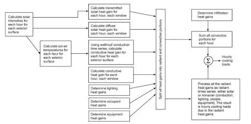 Figure 2: RTS Calculation Schematic [1]
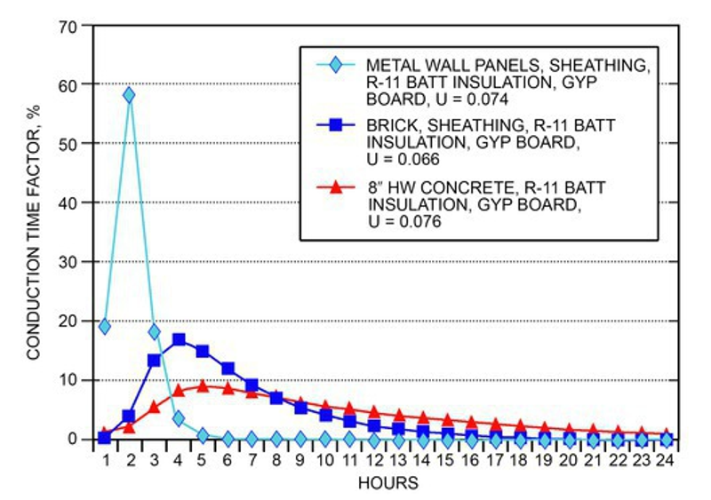
Figure 3 below shows a graphical representation of what the CTS time delay looks like when computing the loads at different hours. It is essentially showing that loads from several hours ago may have an impact on the current cooling requirements. This is a method of estimating the heat absorption of building material in the HB method by using simple empirical data rather than complex calculations of heat absorption. Figure 4 shows the same concept, but for the RTS, non-solar time delay effect. This is a simple linear transformation of the hourly loads by using empirical data, rather than considering the radiant exchange of every surface in the room and solving a large system of equations simultaneously.
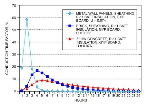 Figure 3: Conduction Time Delay for Different Wall Types [1]
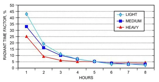 Figure 4: Time Delay of Radiant Heat Gains [1]
The HB method is derived mathematically, and describes the exact process for computing cooling loads, with the exception of not modelling air movement. Air movement can be modelled with computational fluid dynamics (CFD) software, however, it is time-consuming and expensive. Using CFD software in conjunction with software to compute cooling loads using the HB method can become incredibly time consuming and expensive, as well as requiring highly skilled and specially trained users.
The CLTD method is okay at estimating loads, but as systems get more complex, it will typically overestimate the loads and is not as scalable as RTS. CLTD is easy to program into a spreadsheet, but it cannot compete with the accuracy of modern commercial software using the RTS method.
RTS is like the halfway point between the excessively complicated HB method and the outdated CLTD method. With today’s computers and the amount of time engineers can afford to spend on using HVAC load software, RTS is the best of both worlds. RTS uses empirical data to essentially achieve what the HB method aims to achieve, but by using linear transformations rather than computing large matrices of equations simultaneously. With more powerful computing, you can avoid having to let your computer run a simulation for several minutes and instead see the impacts of various architectural features quickly.
[1] American Society of Heating, Refrigeration, and Air Conditioning Engineers. 2021. “Chapter 18: Nonresidential Cooling and Heating Load Calculations.” In 2021 Fundamentals Handbook. Atlanta, GA: American Society of Heating, Refrigeration, and Air Conditioning Engineers.