This article breaks down the process of an energy load analysis to determine the financial effect of improving attic insulation in a home. The goal was to ultimately determine the payback period of such a decision. A single, two-storey house was examined, and a payback period was determined for two scenarios: one where the house was located in a very cold climate, and another where it was located in a milder climate.
The study focused only on heating energy, but similar methodology can be used to study cooling energy performance and payback period.
| Input | Value | Units |
|---|---|---|
| Floor Area | 1,190 | ft2 |
| Storeys | 2 | - |
| Year of Construction | 1950 | - |
| Wall Insulation R-value | 20 | |
| Total Wall Area | 2,000 | ft2 |
| Glass U-value | 0.5 | |
| Total Window Area | 133 | ft2 |
| Basement Area | 600 | ft2 |
| System Type | Gas furnace | - |
| Roof Area | 600 | ft2 |
Ventilation and infiltration were calculated using the automatic calculation tool in HeatWise, resulting in 30 cfm of summer infiltration, 138 cfm of winter infiltration, and 66 cfm of ventilation.
The purpose of the study was to determine the effect of adding roof insulation. The roof was assumed to be at an R-value of R-20 initially, and the new value would be brought to R-40, doubling the total insulation.
The two locations studied were:
| Location | Winter Design Temperature (deg. F) |
|---|---|
| Winnipeg, MB, Canada | -31 |
| San Francisco, CA, USA | 40 |
Load calculations were run on each scenario of location and roof R-value, although when examining only heating costs it is not necessary. Since we are only looking at an analysis on the roof, we can isolate it and study the conduction through the roof, taking net energy lost during the course of a year based on weather data. The conduction heat transfer equation is simply . Where U is the U-value (1/R-value), A is the area, and is the temperature difference from outside to inside.
In this example, A is constant at 600 ft2. U changes between the two roof insulation values, and changes between the two locations. The conduction equation across the roof provides the following values based on design-day outdoor temperatures, and assuming an indoor temperature of 70oF.
| Scenario | Heat loss (Btu/h) | Full House Heating Load (Btu/h) |
|---|---|---|
| San Francisco, R-20 Roof | 900 | 15,284 |
| San Francisco, R-40 Roof | 450 | 14,749 |
| Winnipeg, R-20 Roof | 3,030 | 53,563 |
| Winnipeg, R-40 Roof | 1,515 | 55,381 |
Clearly from the conduction equation heat transfer is directly proportional to the temperature difference across the roof. In each scenario taken isolated from the others, both U and A remain constant, meaning that heat transfer is only dependent on the outdoor temperature (assuming indoor temperature is maintained at a constant setpoint).
The way annual energy analyses are performed is by using the Heating Degree Days (HDD) value available in ASHRAE weather data.
If we assume that the house needs to be heated whenever outdoor temperature is below 65oF, then we can use the the HDD65 value to estimate the number of days degrees Fahrenheit difference from 65. By taking this value and multiplying by 24 to get the heating degree hours value, we have a total combined time and temperature difference value that we can use for annual heating energy usage. For San Francisco the HDD65 value is 2,606 and for Winnipeg it is 10,177. Using this value changes the conduction equation to
The results for just the roof for each scenario are summarized below
| Scenario | Heating energy (Btu) |
|---|---|
| San Francisco, R-20 Roof | 1,876,320 |
| San Francisco, R-40 Roof | 938,160 |
| Winnipeg, R-20 Roof | 7,327,440 |
| Winnipeg, R-40 Roof | 3,663,720 |
Ultimately the goal of this analysis is to determine the payback period of adding insulation to the attic to bring it from R-20 to R-40. Based on current blow-in insulation costs, it can be reasonably estimated that adding an additional R-20 layer of insulation to a 600 ft2 attic would cost approximately 150 to rent the insulation blower, bringing the total to $750.
This example assumes a high-efficiency gas furnace (95% efficiency), and natural gas prices are assumed to be 0.110 per cubic meter in San Francisco. At standard conditions one cubic foot releases 1,038 Btu of heat (), therefore of heat.
Total cost of gas for heat can be calculated with the following equation
Where is the rate charged by the utility (cost per cubic meter of gas) and is the heat released by natural gas (Btu/m3 gas).
Running this calculation for each scenario yields the results in the table below (results are per year).
| Scenario | Heat lost through roof (Btu) | Cost of heat lost through roof ($) |
|---|---|---|
| San Francisco, R-20 Roof | 1,876,320 | $5.97 |
| San Francisco, R-40 Roof | 938,160 | $2.96 |
| Winnipeg, R-20 Roof | 7,327,440 | $15.78 |
| Winnipeg, R-40 Roof | 3,663,720 | $7.89 |
The final calculation is the payback period. Payback period is calculated as initial cost / annual savings. This is based on the difference in annual heating costs from R-20 to R-40. With an initial cost of $750, this results in a payback period of 95 years in Winnipeg and 253 years in San Francisco.
The payback period for both locations was extremely high, indicating that the upgrade in insulation likely is not worth doing.
This could easily be predicted by the load charts displayed in the HeatWise load calculation results. Below is the breakdown of components contributing to the heating load in the Wnnipeg example with R-20 roof insulation. Even before upgrading the insulation, the roof only contributed 5% of the total heating load.
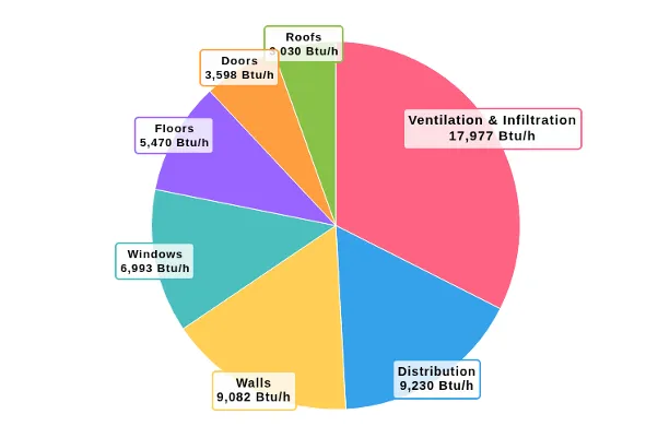
Using the load breakdown in HeatWise can help inform on decisions about where you’re likely to see a return on investment from home upgrades. In this example, investing in preventing air leakage and potentially getting an HRV would make a much bigger difference considering that ventilation and infiltration accounted for 32.5% of the heating load - 6x more than the roof load.